

Project management has an odd habit: many activities are treated as useful almost by default, while the moment they happen is usually chosen either by ritual or by accumulated team irritation. Meetings, syncs, reviews, clarifications, retrospectives—all of them have long become part of normal work. But the need for such events is rarely derived from the internal logic of the project itself.
And yet every intervention has a cost. It takes time, pulls people away from productive work, increases organizational overhead, and often slows the project down. So there should be a substantive reason for it: why this intervention is needed here, why now, and why at this scale.
What follows is one way to derive such interventions from the nature of project work itself.

This text can be read on its own. It is aimed at practice rather than theoretical debate. The theoretical foundation of the approach was outlined in the earlier articles of this series—on classification, principles, causes, and project thermodynamics—but here the focus is mainly on the applied side of the method.
Like any new concept, this approach is open to criticism and does not claim to be final. What follows is simply its working presentation in a simplified form.
Contents
- Where Project Temperature Comes From
- Productive and Management Activities
- The Simplified Method
- Overheating and Cooling
- Overcooling and Initial Heating
- Project Segmentation
- Calibration on Scrum
- Limitations of the Method
- Practical Usefulness
- What Comes Next
Where Project Temperature Comes From
Every task in a project adds uncertainty to its overall state. That uncertainty may appear as hidden defects, distorted understanding, accumulated delays, overspending, and other consequences that are not always visible when they first arise.
This uncertainty is probabilistic. A particular error may never materialize, a defect may never surface, and a local misunderstanding may not immediately lead to failure. But as the project develops, such probabilities accumulate. At some point, the presence of undetected defects, semantic distortions, and hidden losses has to be treated not as an exception, but as a working assumption.
As this accumulation continues, local uncertainty stops being merely local. Separate episodes begin to affect the condition of the project as a whole. That makes it useful to evaluate them not only one by one, but also through an aggregate indicator of total uncertainty.
That indicator will be called project temperature—the overall level of accumulated uncertainty that describes the state of the project as a system.

An immediate clarification is important here: temperature is not meant as a physical equivalent. It is a practical engineering metric, useful for comparing project states and choosing the right moment for management intervention.
The analogy comes from thermodynamics. In this model, the local uncertainty of an individual task corresponds to the amount of heat the task introduces into the system, while the overall state of the project corresponds to the system’s temperature. The factor that links local uncertainty to the global state can naturally be interpreted as the project’s heat capacity.
If we follow the analogy further, project heat capacity, like physical heat capacity, depends on two components: the scale of the system and its internal properties. In project terms, those components can be approximated by team size and process maturity.
At an intuitive level, this makes sense. The larger the system, the harder it is for the same impact to noticeably change its overall state. In the same way, the same mistake usually causes less overall destabilization in a larger, more organized team than in a smaller or less mature one.
We can define project temperature as:
$$ T_p = k \cdot \sum \left(\frac{Q_m}{C_t}\right) $$
where $Q_m$ is the heat contributed by an individual task, $C_t$ is the heat capacity of the project team, and $k$ is a normalization coefficient that sets a convenient temperature scale.
The value of $Q_m$ can be estimated through the normalized standard deviation of a task’s PERT estimate:
$$ Q_m = \left(\frac{\sigma}{d}\right)^2 $$
where
$$ \sigma = \frac{P - O}{6} $$
Here, $O$ is the optimistic estimate, $P$ is the pessimistic estimate, and $d$ is the length of a working day.
The heat capacity of the project team can be estimated as:
$$ C_t = N \cdot L $$
where $N$ is the weighted team size at the time the task is performed, and $L$ is the relative maturity level of the team.
Substituting this into the temperature formula gives:
$$ T_p = k \cdot \sum \left(\frac{Q_m}{N \cdot L}\right) $$
If we assume that team maturity changes slowly within a single project, then $L$ can be taken outside the summation:
$$ T_p = \frac{k}{L} \cdot \sum \left(\frac{Q_m}{N}\right) $$
In this form, $L$ is best understood as a scaling factor for the execution environment. The higher the maturity, the less strongly the same local uncertainty affects the overall state of the project.
There is one important caveat. In this version of the method, $L$ should be understood primarily as a practical environmental coefficient rather than as a precisely measured objective quantity. Its estimation is inevitably approximate and based on accumulated experience. That is why the method aims not at absolute precision, but at comparability of results. At the same time, repeated use of the method can gradually refine $L$, since it makes it possible to track changes in team maturity across projects.
Productive and Management Activities
In the proposed model, all project activities are divided into productive and management activities.
Productive activities directly create product value, but at the same time they also increase uncertainty. Part of their effect is inevitably accompanied by internal “heating” of the project.
Management activities do not create product value directly. Instead, they influence the product through organization, coordination, and correction of the productive process. During such activities, the related productive work is usually fully or partially paused. That is why management activities naturally define the boundaries of project segments.
In the full version of the model, the effect of such interventions is evaluated with regard to their local scope, the composition of participants, and the loss of efficiency that comes with collaborative work. But for practical use, it makes sense to begin with a simpler scheme.
The Simplified Method
The simplified version requires only three kinds of input data: the optimistic estimate $O$, the pessimistic estimate $P$, and the size of the project team at the relevant stage. In most projects, that is enough even with only minimally organized tracking.
Using this version does not require special software or any major restructuring of the planning process. Standard tools that already record task estimates and team composition are sufficient.
For each productive activity, its contribution to project temperature growth is calculated at the planning stage as:
$$ T_i = \frac{k \cdot (P - O)^2}{36 \cdot d^2 \cdot N} $$
where $O$ is the optimistic estimate of the task, $P$ is the pessimistic estimate, $d$ is the length of the working day, $N$ is the project team size during execution, and $k$ is the normalization coefficient.
In the baseline version of the simplified method, we take:
$$ k = 725 $$
This number should not be treated too literally. $k = 725$ is not a fundamental constant of the model, but a calibration coefficient derived from a reference Scrum scenario. In other fields and for other kinds of projects, it may need adjustment.
The sum of all $\sum_{i=1}^{n} T_i$ values across tasks forms the project’s cumulative temperature profile, rising as productive activities are completed.
 To make practical tracking easier, one can introduce a notional resource called project temperature and assign it to tasks in the amount of $T_i$. The accumulation profile of that resource then becomes a visible indicator of the project’s condition.
Overheating and Cooling
The next step is to determine the temperature level at which a project begins to lose controllability. This threshold can be estimated either from expert observation or from the experience of previously completed projects.
If such a threshold is not predefined, it can be refined during execution. In practice, a common sign of overheating is the growth of uncoordinated horizontal coordination: the team spends more and more time discussing what is happening among themselves, while becoming less and less capable of turning those discussions into clear management decisions.
As a reference point, let us define project overheating as 100 °M and treat that value as the project’s “boiling point.” The coefficient $k$ is then selected so that the scale of the model corresponds to that level. From an engineering perspective, it is reasonable to keep some safety margin and take 80 °M as the upper boundary of acceptable working temperature.
A fair caveat is necessary here: 100 °M, 80 °M, and later 30 °M should all be understood as calibration reference points of the first version of the model, not as universal constants valid for every project.
Planning should therefore aim to keep the temperature profile within the working range.
When project temperature approaches 80 °M, a management activity should be introduced. In the simplified model, this corresponds to reducing the temperature by:
$$ T_{ic} = T_p \cdot \left(1 - \frac{1}{\sqrt{N_c}}\right) \cdot F_t $$
where $T_p$ is the current project temperature, $N_c$ is the number of participants in the management activity, and $F_t$ is the duration coefficient: for activities shorter than one hour, it equals the fraction of an hour represented by their duration; for activities lasting one hour or longer, it is taken as one.
This is a deliberate simplification. Here, the management intervention is assumed to affect the project as a whole rather than a local area of uncertainty. In the full version, this assumption is removed.
The resulting value defines the amount of cooling, changes the project’s temperature profile, and helps identify the most appropriate moment for the next intervention.
As with productive tasks, this change can be tracked through a separate notional resource that records temperature reduction.
In other words, the final profile in the simplified model is built as the difference between accumulated heating and accumulated cooling.
Overcooling and Initial Heating
When planning management activities, it is important to remember that overcooling a project is undesirable too. Usually, it means that too much effort is being spent on meetings and coordination with too little return.
If management activities do not lead to substantive decisions, and their outcome repeatedly collapses into “we continue following the plan,” then this is no longer management but an excess of it. In that situation, it makes sense either to reduce the frequency of such activities or to narrow the circle of participants.
It is also important not to assume zero temperature at the start of a project. In reality, the initial state almost always already contains uncertainty—both in the product itself and in the team’s understanding of how it should be implemented. As a practical estimate of initial heating, one can take a level of about 30 °M.
This is a practical starting heuristic, not a universal norm. Its usefulness lies in preventing the model from replacing a real, imperfect beginning with the fiction of a perfectly defined starting point.
Project Segmentation
Management activities divide a project into segments within which it becomes possible to control the accumulation of uncertainty and account for aggregate risks in schedule, cost, and quality. In that way, the project can be kept within its working range.
Yes, this form of management increases project duration and cost. But that additional price is not paid for bureaucracy. It is paid for keeping risks within acceptable bounds and preserving stable product quality relative to the resources spent.
One of the more important consequences of the method is that it helps reveal the internal structure of a project—its topology of uncertainty. In this sense, we are dealing with an invariant defined not by calendar scale or absolute duration, but by the configuration of tasks and the relationships between them.
This idea, however, should be treated cautiously. The hypothesis of uncertainty topology is still exploratory and requires further validation across series of real projects. Even in its current form, though, it already suggests one useful practical conclusion: project segmentation can be derived not from calendar rhythm as such, but from the pace of uncertainty accumulation.
Calibration on Scrum
After the full version of the model had been developed, it was implemented in a project management application. On that basis, a project corresponding to a typical Scrum setup was simulated: a recommended team composition, three two-week sprints, a full set of regular management activities, and a test production workload.
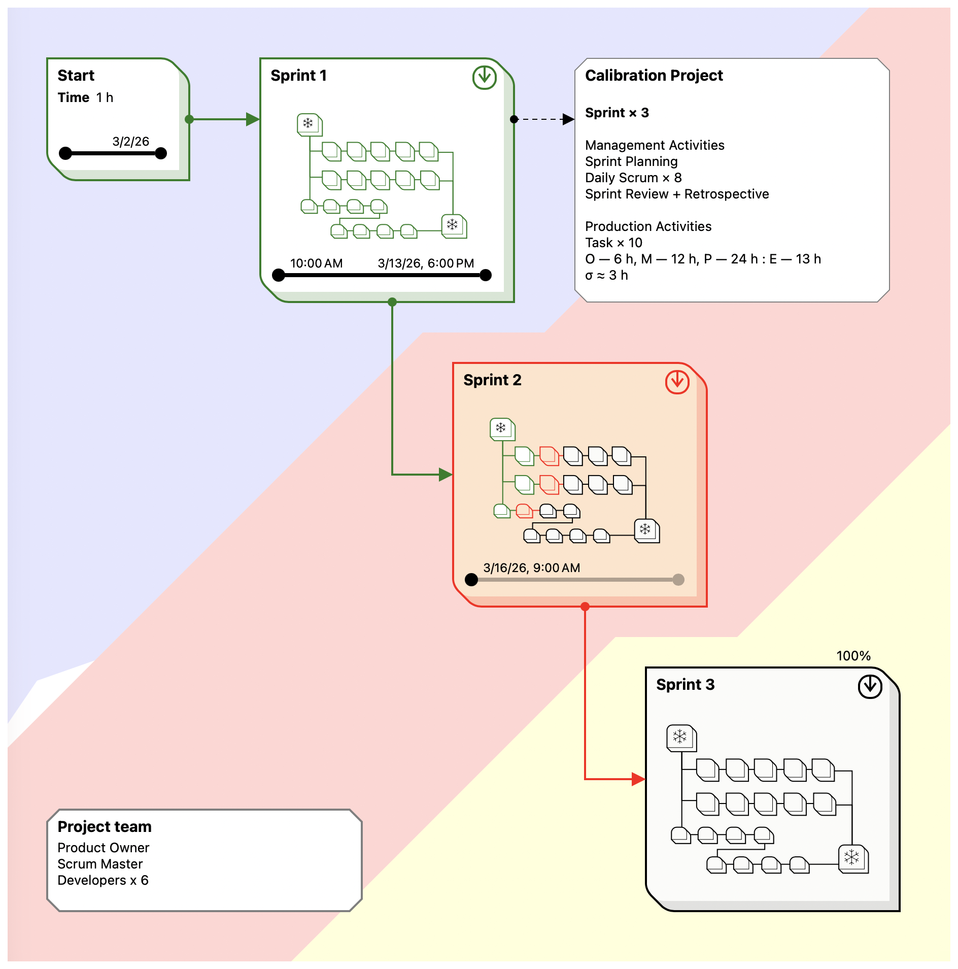

Scrum was chosen as the calibration environment for a simple reason: it is sufficiently formalized and provides a stable reference structure for calculations, from team composition to the set of regular management events. In addition, the parameters of typical tasks in such an environment are better understood than in many other project scenarios.
The coefficients were calibrated under the condition that project temperature in normal working mode should not exceed 80 °M.
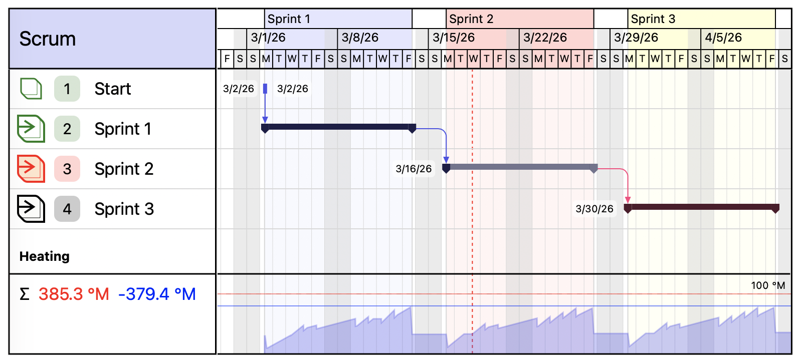
The calculation showed that in a typical Scrum project built according to the recommended rules, one sprint generates roughly the same amount of uncertainty that is later compensated by management activities. As a result, the temperature profile takes on a clearly cyclical form. This fits well both with the internal logic of the model and with the observable rhythm of Scrum projects in practice.
It is important to stress that this is not a mathematical proof of Scrum’s universal stability. It is merely the result of a calibration scenario. But the conclusion is still useful: through this lens, Scrum appears not simply as a set of rituals, but as a regime for regularly draining accumulated uncertainty.
The same project was also calculated in parallel using the simplified method. The results turned out to be close: the deviation from the full model was about 15%. On that basis, the recommended coefficient $k$ for the simplified version was selected.
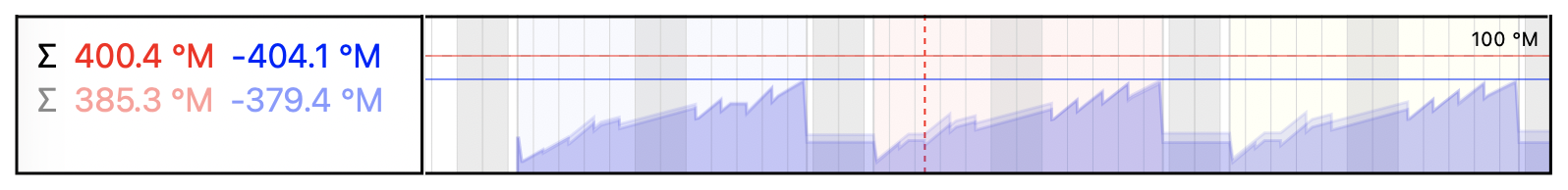
This result should not be overstated either. For now, it is an encouraging but still local outcome of one particular scenario. Even so, it suggests that the simplified version is useful as a practical tool, not merely as an illustration.
The virtual experiment also showed that the method has a degree of robustness to inaccurate estimates. Overestimating the rate of uncertainty accumulation is often accompanied by overestimating the expected effect of management activities, so in practice these deviations partially compensate for each other. That means the model can still produce a project profile reasonably close to the observed one, even when the input data is incomplete, and can still help reveal the project’s internal structure.
Limitations of the Method
The method works less well for tasks in which time uncertainty is not the main carrier of risk. This applies, for example, to work with fixed deadlines, where variability shifts instead into final quality or cost.
In such cases, the basis for calculation should not be temporal uncertainty, but the relevant domain uncertainty: standard deviation in quality, cost, or some other parameter that actually carries the main risk. In other words, the method is tied not to schedule as such, but to the parameter through which uncertainty genuinely manifests in the task.
The method is also not designed for dominant management systems where the correctness of a decision is determined not by the quality of comparison among alternatives, but by the position of the person making or framing the decision. Where there is no real competition of viewpoints, the logic of corrective management activities becomes less effective.
In addition, the coefficients used here were derived in the context of the IT sector and cannot simply be transferred unchanged to other industries. This is especially important in environments where the main uncertainty is tied not to intellectual coordination but to material production. In such cases, the scales and normalization coefficients will likely require separate calibration.
In essence, the method assumes an environment in which uncertainty is genuinely processed through comparison, discussion, and correction, rather than suppressed by status or rigid technological inertia.
Practical Usefulness
One of the method’s practical advantages is that it provides a substantive justification for introducing management activities in a targeted way. They stop looking like obligatory rituals imposed by external doctrine and begin to look like a natural response of the project to accumulated uncertainty.
This becomes especially clear in flexible approaches: artificial rhythmic segmentation can be reinterpreted as segmentation emerging from the project’s real risk profile.
Management activities are also convenient as anchor points for segmentation. Through them, it becomes possible to identify the project’s actual structure and build segmentation that corresponds not to a formal work rhythm, but to the real distribution of uncertainty and risk.
The method also makes it possible to analyze the profiles of different project branches separately. That helps avoid mixing independent streams of work and makes it easier to isolate the most risk-heavy areas in time.
Finally, even in simplified form, it helps choose a reasonable scale for management interventions. Even here, one conclusion is already visible: the narrower the scope of issues under consideration and the more precisely the moment of intervention is chosen, the lower the overhead while preserving the effect.
In the end, the method helps not only measure project overheating, but also gradually localize its source.
What Comes Next
The simplified version is convenient as a practical working tool, but in large projects its precision becomes insufficient. It does not account for the local nature of some management interventions, the different roles of participants, the loss of efficiency in collaborative work, or the number of tasks that simultaneously fall within the area under discussion.
All of these refinements belong to the full version of the model and require separate discussion. That is also where more precise estimates appear for scope of impact, participant composition, and the real effectiveness of meetings.
But even in simplified form, the method already solves the main problem: it links management interventions not to ritual, but to the accumulation of uncertainty. That alone is enough to look differently at project segmentation—and at the very moment when a project actually needs management.
In that sense, the method shifts the focus from managing tasks to managing the state of the project. Within this logic, temperature, segmentation, and management activities are linked not formally, but causally. That is precisely what makes the approach useful: it helps explain when a project really needs management, where it is needed, and what scale it should take.
The next article will walk through the full project workflow, including segmentation in practice and thermodynamic analysis.